
Processing LIDAR data using a Hough Transform
1. Overview
Once we got the robot to read the LIDAR data successfully, we needed to process the data in order to use it to determine the robot’s position. With our 4-walled rectangular field, we expected to use the readings of the walls to determine the robot’s most likely position and orientation.
2. Original Plan
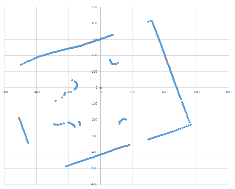
The original plan was to use a Least-Squares Linear Regression to convert the point cloud generated by the LIDAR into a series of lines. LSLR is used commonly in statistics and is very simple and fast from a computation standpoint. However, it is highly suceptible to outliers and would require filtering to isolate the set of points belonging to each wall beforehand. Therefore, we determined it wouldn’t be an ideal solution. Neither of us had experience with image analysis or feature abstraction, so we didn’t know of any alternatives.
3. Hough Transform
After some more research, we decided that a Hough transform would be an excellent candidate for detecting the lines of our track boundary. A classical Hough transform (as opposed to the more complicated general version) essentially creates a distribution (called the Hough space) that represents the liklihood of any given line being represented in the image (or point-cloud in our case). For the ease of calculation and for its independence from the standard basis (coordinate axes), we parameterize these lines in terms of \(r\) and \(\theta\). After searching for a simple and easily accessible Hough transform algorithm written in C, we decided to write the algorithm from scratch.
Line Parametrization: \[x \cos \theta + y \sin \theta = r\]
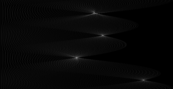
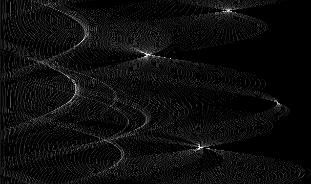
To ease in visualization, we also wrote a function that would convert the Hough space to a bitmap image (specifically a grayscale NetPBM) that could be visualized. The image is a graph of \(r\), on the x-axis, measured in millimeters, versus \(\theta\), on the y-axis, measured in degrees. Thus, each pixel in the image represents a potential line represented in the point cloud. The darker the pixel, the more likely the line.
In the following examples, the image of white on black is the visual representation of the Hough space. The x-axis represents distance, with 1 mm = 1 pixel and the y-axis represents the angle with 1 degree = 1 pixel. The brightness at each point is directly proportional to the probability of a a parametric line existing with those parameters.
Hough Transform Example with Clean Field Data

Hough Transform Example with Impure Field Data
4. Line detection and positioning
From the hough transform, it is not too difficult to detect lines. Our algorithm starts by finding the brightest point, which it assumes to represent one of the walls of the field. Then, it searches for the three other most likely lines at 90 degrees, 180 degrees, and 270 degrees. To determine positon using these lines, we find the perpedicular lines parallel to the field axes running through the origin (our robot’s position). Then, we calculate the field center. Next, by applying a linear transformation, we orient the robot on the field’s coordinate system. Finally, we calculate the most likely angle orientation based on the previous iteration’s results.